WILL Part I: Relational Geometry
*Interactive page — highlight any text to ask WILL AI for an explanation.*
What is This Page?
This page transparently demonstrates how the laws of Special and General Relativity inevitably arise from a single principle of reduction, pure logic, and geometry. By revealing their fundamental essence, it offers elegant solutions to many long-standing problems in physics. Through simple and clear numerical calculations of well-known phenomena, this narrative will show not only that the Universe is, at its core, incredibly elegant and simple, but also that fundamental physics is accessible to any dedicated seeker, regardless of their level of mathematical perversion.
For full mathematical derivations:
For unique testable predictions:
For questions and curiosity:
▶ Quick Glossary: Key Terms & Concepts
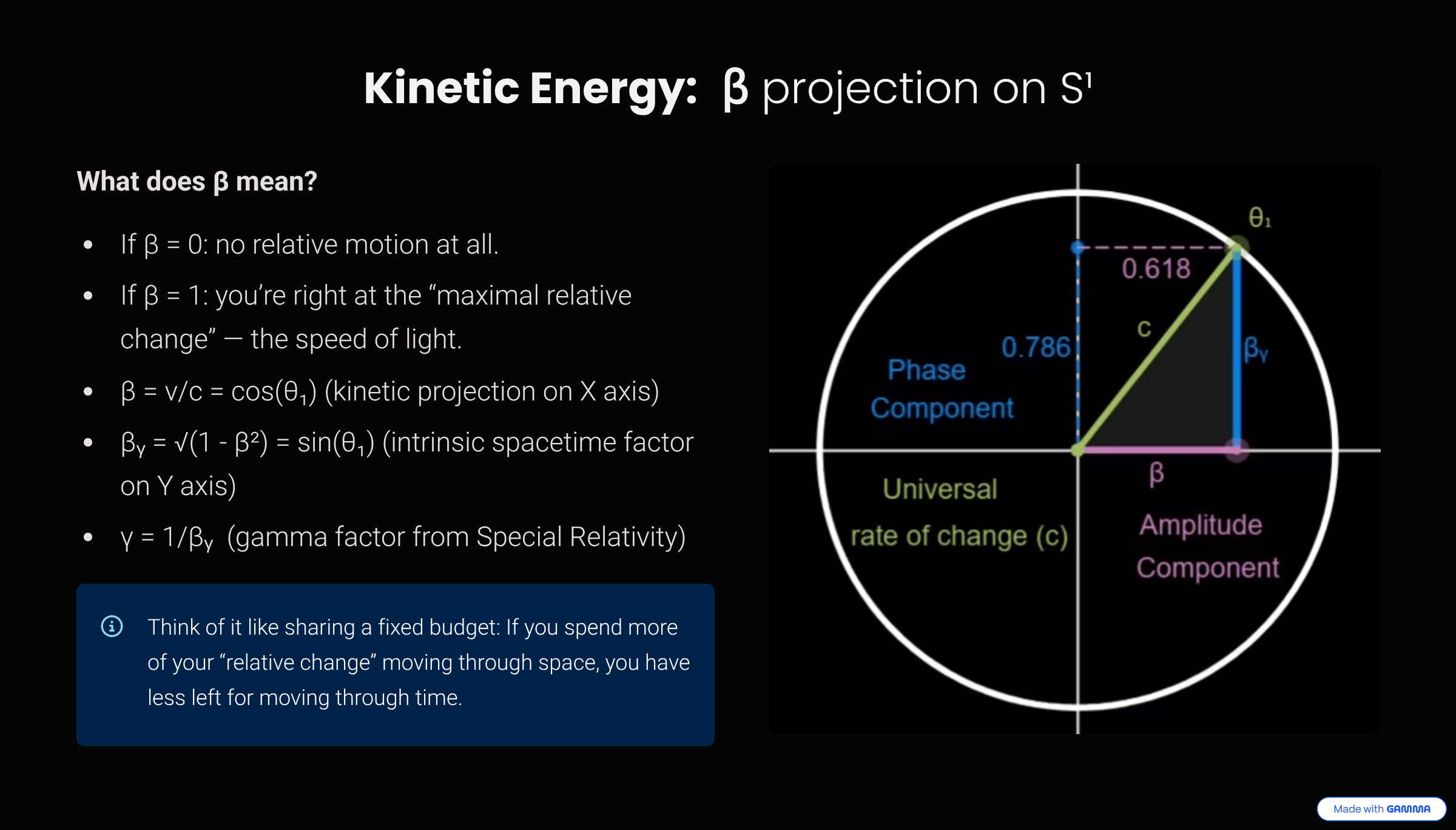
Beta (β): The kinetic projection. Representing the ratio of an object's velocity to the universal rate of change (β = v/c). It quantifies how much of the "speed of change" is perceived as motion through space relative to observer. Not an intrinsic property of an object but rather a measure of the differences between states, perceived from the perspective of an observer.
Kappa (κ): The potential projection. It measures how deeply an object is situated within a gravitational field, relative to an observer, and asociated with escape velocity (κ = v_e/c). It indicates proximity to an event horizon, at κ = 1 object has to move with the speed of light (c) in order to escape gravity (event horizon). Not an intrinsic property of an object but rather a measure of the differences between states, perceived from the perspective of an observer.
Universal rate of channge (c): Another name for the speed of light, viewed here as the fundamental, invariant tempo of change in the universe. It is not merely the speed of light but the constant rate at which all energetic interactions and transformations occur, speed limit for any change or information transfer.
Epistemological Hygiene: The principle of removing all unnecessary assumptions when building a theory, using only what’s logically required (nothing extraneous).
Event Horizon: The boundary around a black hole beyond which nothing can escape. (At this “point of no return,” the escape velocity equals the speed of light.)
Photon Sphere: A region near a black hole (about 1.5 times the Schwarzschild radius) where light can orbit in a circle if moving tangentially. It's an unstable orbit – light can fall in or escape if perturbed.
Critical Density: The maximum energy density that can can be packed into a given radius, dependent on central mass and the distance from it center. It increases closer to a central mass but never becomes infinite, thus preventing the formation of infinite densities (singularities).
Singularity: A point of infinite density where conventional physics breaks down. Standard GR predicts singularities (e.g. inside black holes); WILL Geometry avoids them by enforcing a finite critical density.
Energy–symmetry Law: The rule that energy differences always balance out between perspectives. If one observer sees a gain, another sees an equal loss — preventing any “free” energy or causality violations (this also ensures a universal speed limit).
This page explores a foundational model of physics built from a single principle. Instead of describing observed phenomena with external laws, it generates the laws of physics as an inevitable consequence of that principle.
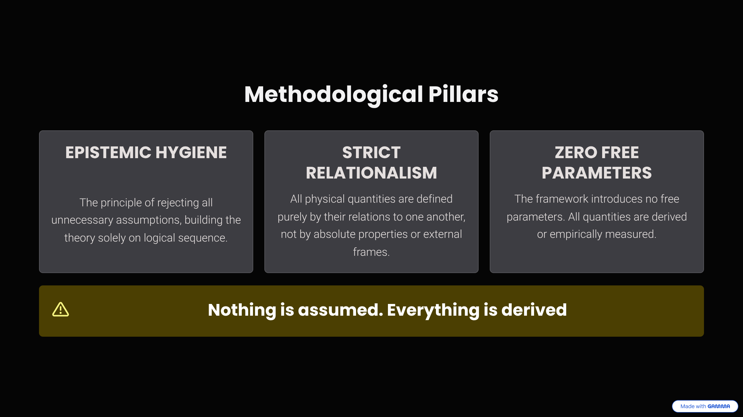
To construct a theory from a single idea without introducing new postulates requires an uncompromising methodology. These pillars serve as the logical rules that guide the entire framework, ensuring no hidden assumptions or arbitrary constants are smuggled in.
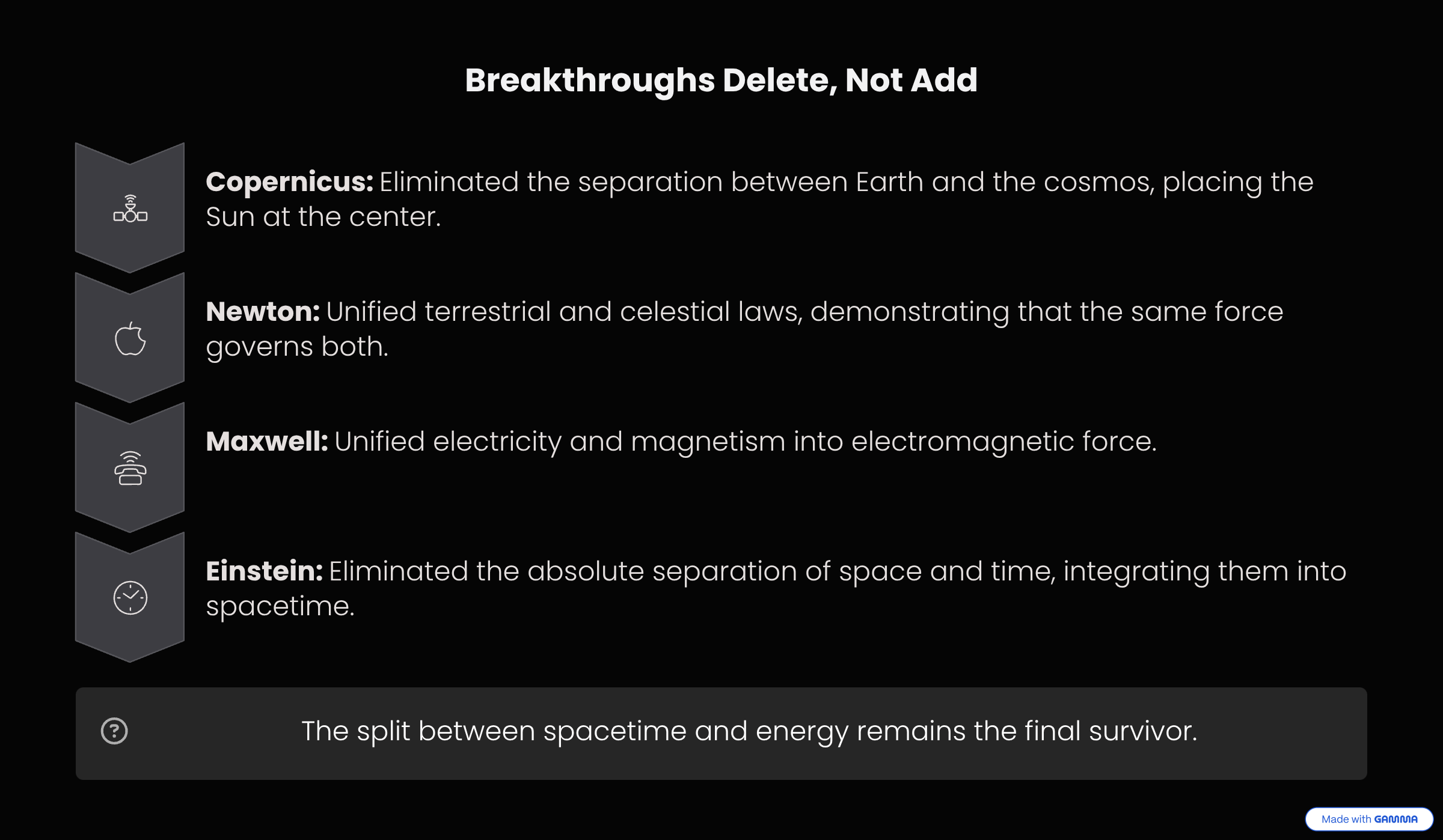
This approach follows a powerful historical pattern. The greatest leaps in physics have consistently come not from adding new entities, but from removing a false separation. Just as Copernicus removed the Earth/cosmos divide and Einstein unified space and time, this framework targets the final, unexamined split in modern physics.
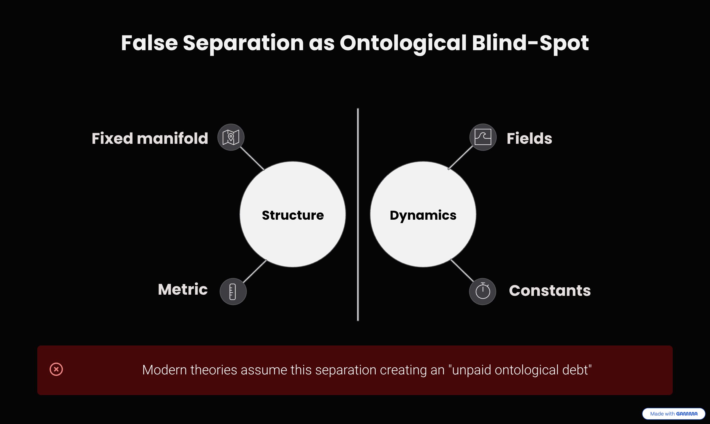
The contemporary split is between the structure of the universe (a fixed stage, or manifold) and the dynamics that unfold upon it (fields and energy). This separation is not an empirical discovery but an implicit assumption—an "unpaid ontological debt". By removing it, we are forced to identify geometry and energy as two aspects of a single entity.
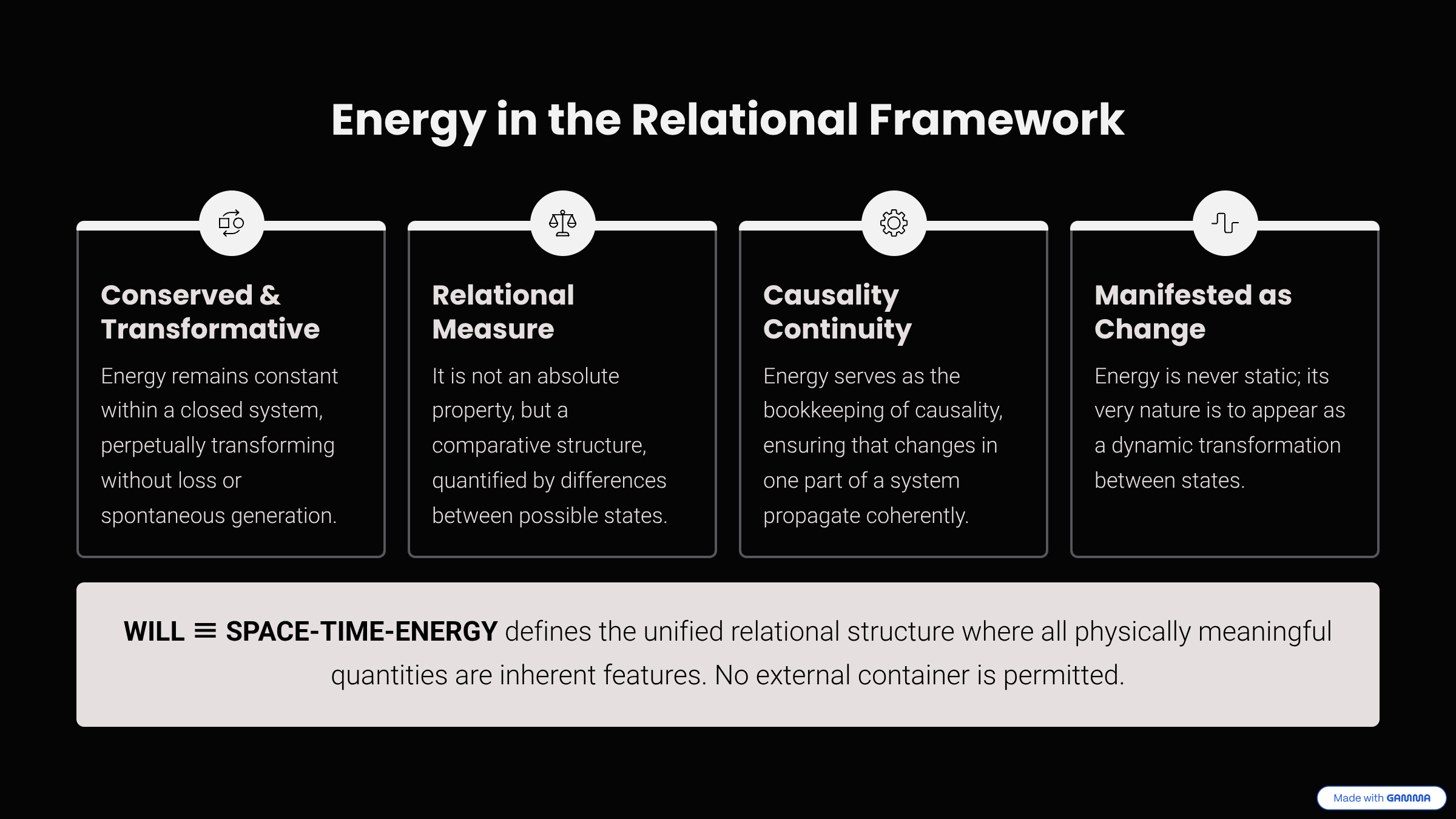
Energy is the relational measure of difference between possible states, conserved in any closed whole. It is not an intrinsic property of an object, but comparative structure between states (and observers), always manifesting as transformation.
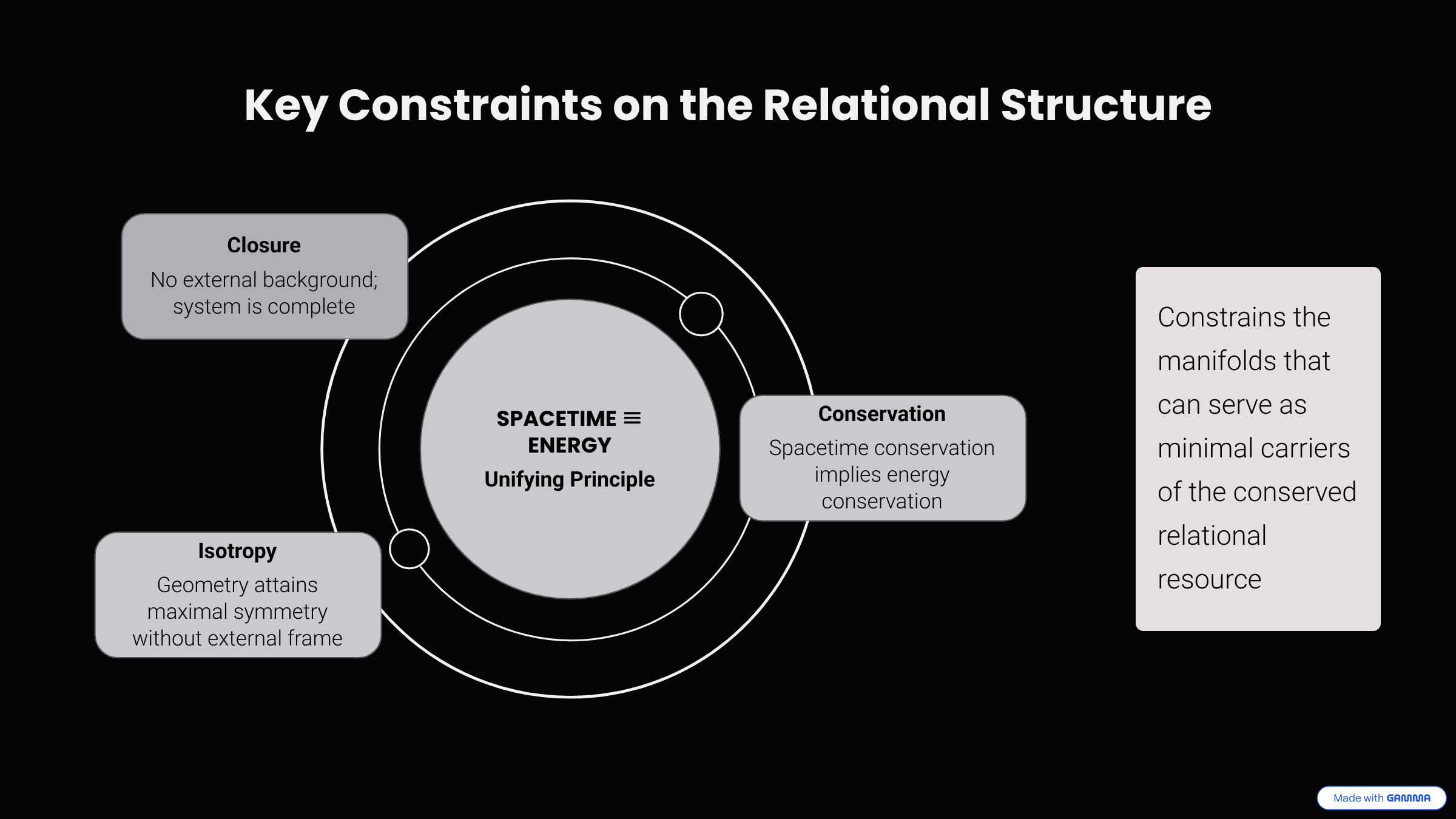
These three constraints—Closure, Conservation, and Isotropy—are immediate, unavoidable consequences of a universe built from a single, self-contained principle. The next crucial question is: what mathematical forms can possibly satisfy all these rigid requirements at once?
Lemma: Closure
Under Principle 4.1 (\(\text{SPACETIME} \equiv \text{ENERGY}\)), WILL is self-contained: there is no external reservoir into or from which the relational resource can flow.
Lemma: Conservation
Within WILL, the total relational "transformation resource" (energy) is conserved.
Lemma: Isotropy from Background-Free Relationality
If no external background is allowed, then no direction can be a priori privileged. Thus the admissible relational geometry of WILL must be maximally symmetric.
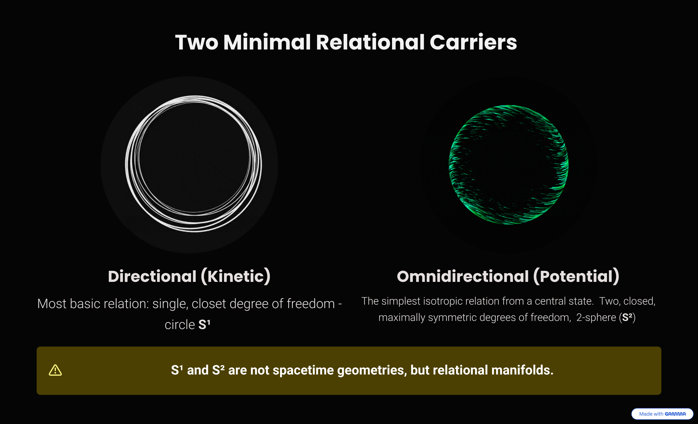
Theorem: Minimal Relational Carriers of the Conserved Resource
The only closed, maximally symmetric manifolds that can serve as minimal carriers of the conserved relational resource are:
- \(S^1\) for directional (one-degree-of-freedom) relational transformation;
- \(S^2\) for omnidirectional (central, all-directions-equivalent) relational transformation.
S¹ and S² are not spacetime geometries, but relational manifolds.
▶ Show Interactive Graph: Kinetic projection β on the Circle S¹ (Desmos)
The Duality of Transformation
Lemma: Duality of Evolution
The identification of spacetime with energy and its transformations necessitates two complementary relational measures:
- the extent of transformation (external displacement), and
- the sequence of transformation (internal order).
Proof
Any complete description of transformation must specify both what changes and how that change is internally ordered. The circle \(S^1\) provides the minimal geometry enforcing such complementarity: its orthogonal projections furnish precisely two non-redundant coordinates.
We define these orthogonal projections as follows:
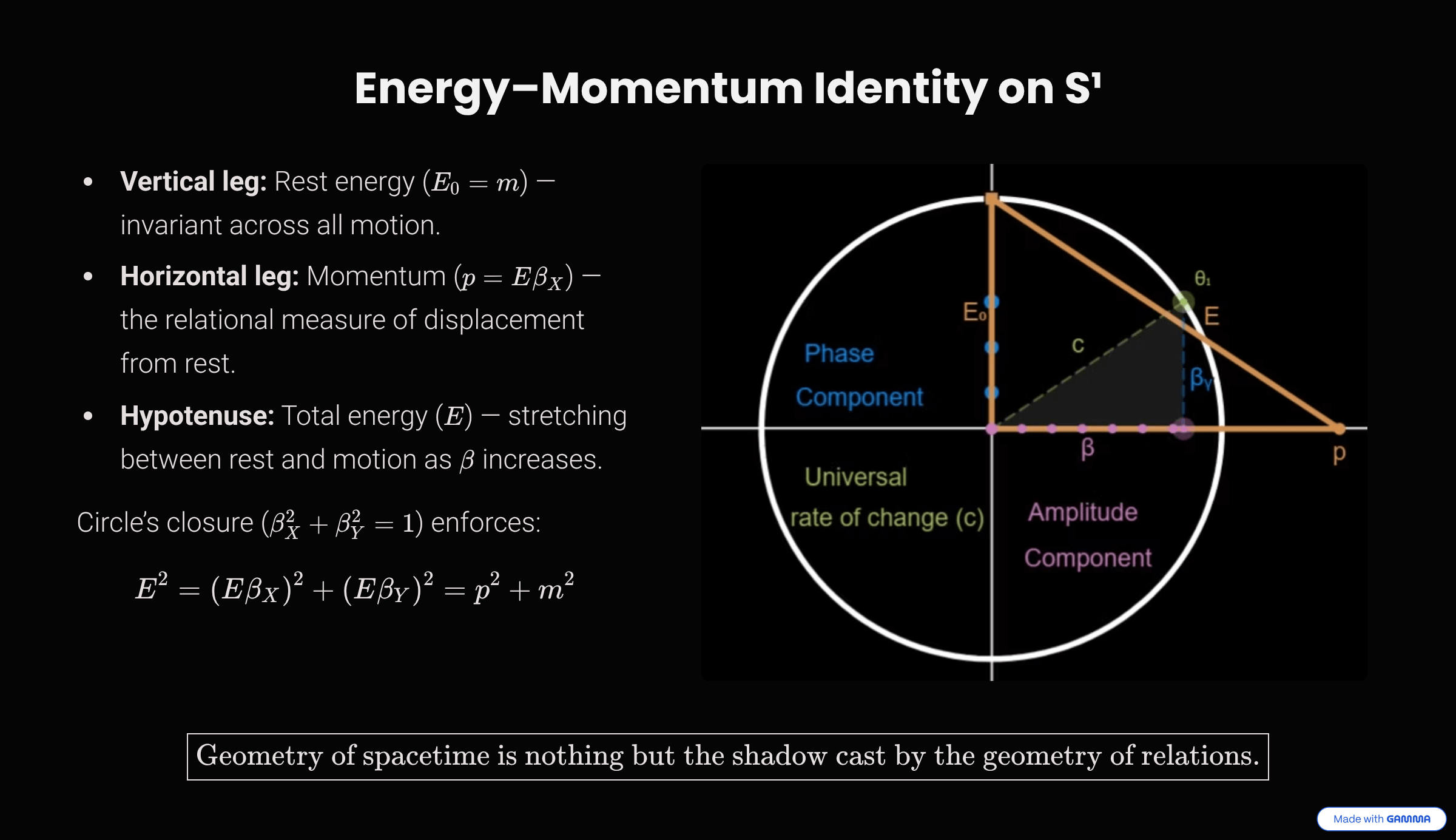
- The Amplitude Component (\(\beta\)): This projection represents the relational measure between the system and the observer. It corresponds to the extent of transformation, which manifests physically as momentum.
- The Phase Component (\(\beta_Y\)): This projection represents the internal structure of a system. It governs the intrinsic scale of its proper space and proper time units. A value of \(\beta_Y=1\) represents a complete and undisturbed manifestation of this internal structure, a state we identify as rest.
Conservation Law of Relational Transformation
Theorem: Conservation Law of Relational Transformation
The orthogonal components of transformation (\(\beta,\beta_Y\)) are bound by the closure relation:
\(\beta^2 + \beta_Y^2 = 1\)
Proof
Since \(S^1\) is closed, every point on the circle is constrained by the Pythagorean identity of its projections. This closure enforces conservation across all processes.
Consequence: Relativistic Effects
Proposition: Physical Interpretation: Relativistic Effects
The conservation law implies that any redistribution between the orthogonal components (\(\beta,\beta_Y\)) manifests physically as the relativistic effects of time dilation and length contraction.
Proof
The components satisfy \(\beta^2 + \beta_Y^2 = 1\). An increase in the relational displacement \(\beta\) enforces a decrease in the internal measure \(\beta_Y\). This reduction of \(\beta_Y\) corresponds to dilation of proper time and contraction of proper length, while the growth of \(\beta\) represents momentum. Thus the relativistic trade-off is the direct physical expression of the geometric closure of \(S^1\).
The geometry of spacetime is the shadow cast by the geometry of relations.
▶ Show Interactive Graph: The Energy-Momentum Triangle (Desmos)
Kinetic Energy Projection on \(S^1\)
Since \(S^{1}\) encodes one-dimensional displacement, the total energy \(E\) of the system must project consistently onto both axes:
\(E_{X} = E \beta_{X}, \qquad E_{Y} = E \beta_{Y}\)
Theorem: Invariant Projection of Rest Energy
For any state (\(\beta, \beta_Y\)) on the relational circle, the vertical projection of the total energy is invariant:
\(E \beta_Y = E_0\)
Proof
When \(\beta=0\), closure enforces \(\beta_Y=1\), yielding \(E=E_0\). Since closure applies for all \(\theta_1\), the vertical projection \(E\beta_Y\) remains equal to this rest value in every state.
Corollary: Total Energy Relation
From the theorem it follows that:
\(E = \frac{E_0}{\beta_Y} = \frac{E_0}{\sqrt{1-\beta^2}}\)
The historical Lorentz factor is the reciprocal of \(\beta_Y\): \(\gamma\) = 1/\(\beta_Y\).
Rest Energy and Mass Equivalence
Corollary: Rest Energy and Mass Equivalence
Within the normalization \(c=1\), the invariant rest energy equals mass:
\(E_{0} = m\)
Proof
From the invariant projection \(E\beta_Y = E_0\) and closure of \(S^1\), no additional scaling parameter is required. Hence the conventional bookkeeping identities \(E_0 = mc^2\) or \(m = E_0/c^2\) reduce to tautologies. Mass is therefore not independent, but the rest-energy invariant itself.
Mass is the invariant projection of total rest energy.
Energy–Momentum Relation
Proposition: Horizontal Projection as Momentum
On the relational circle, the unique relational measure of displacement from rest is the horizontal projection \(E\beta\); hence:
\(p \equiv E\beta \quad (c=1)\)
Corollary: Energy–Momentum Relation
With \(p\) identified by the proposition and \(m=E_0\), the closure identity yields:
\(E^{2} = p^{2} + m^{2} \quad (c=1)\)
Equivalently, upon restoring \(c\):
\(E^{2} = (pc)^{2} + (mc^{2})^{2}\)
Proof
By closure, \((E\beta)^2 + (E\beta_Y)^2 = E^2\). Substituting \(p=E\beta\) and \(m=E_0\) proves the claim. Restoring \(c\) is dimensional bookkeeping: \(p\mapsto pc\) and \(m\mapsto mc^{2}\), while \(E\) remains \(E\), yielding the standard form.
The relation \(E^{2}=p^{2}+m^{2}\) is the geometric identity of \(S^1\).
▶ Show Interactive Graph: Potential Energy projection on S² (Desmos)
With both the kinetic (SR on \(S^1\)) and potential (GR on \(S^2\)) projections defined, we can now compose them. This composition reveals how WILL Geometry derives one of General Relativity's core postulates—the Equivalence Principle—not as an axiom, but as a structural necessity.
▶ Show Formal Derivation of Potential Energy Projection
Analogous to \(S^1\), the relational geometry of the sphere, \(S^2\), provides orthogonal projections for two aspects of omnidirectional transformation. We define them as follows:
- The Amplitude Component (\(\kappa\)): The relational gravitational measure. A value of \(\kappa=1\) corresponds to the event horizon.
- The Phase Component (\(\kappa_X\)): This projection governs the intrinsic scale of proper length and time units.
These components are bound by the conservation law of the closed system:
\(\kappa_X^2 + \kappa^2 = 1\)
Consequence: Gravitational Effects
The redistribution of the budget between the Phase and Amplitude components produces the effects of General Relativity. An increase in the relational measure (\(\kappa\)) requires a decrease in the measure of the internal structure (\(\kappa_X\)). This geometric trade-off is observed physically as gravitational time corrections.
Gravitational Tangent Formulation
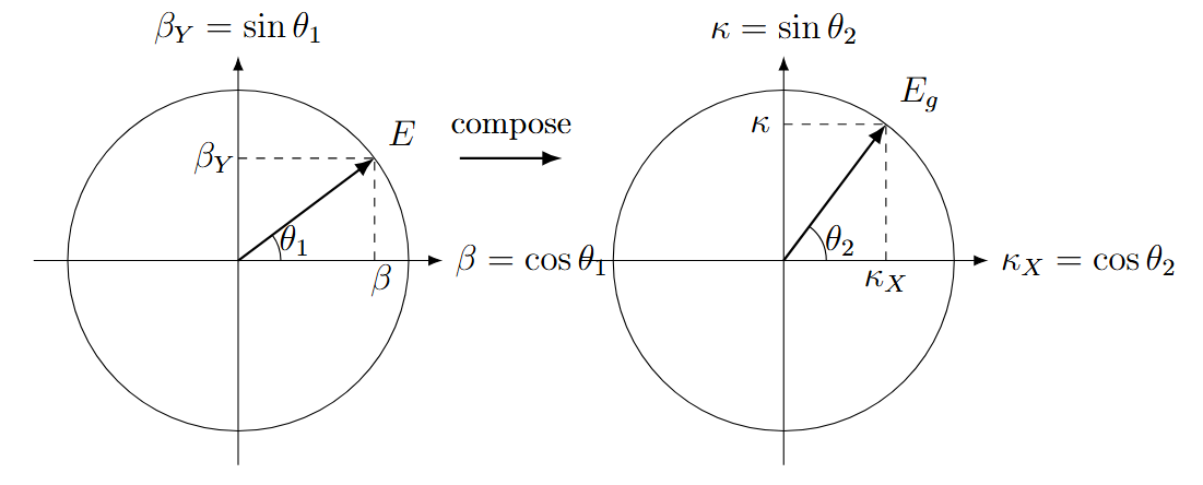
Just as the relativistic energy-momentum relation is expressed via \(\beta = \cos\theta_{1}\), its gravitational analogue follows from \(\kappa = \sin\theta_{2}\). We define the gravitational energy and momentum:
\(E_{g} = \frac{E_{0}}{\kappa_{X}}\) where \(\kappa_{X} = \sqrt{1 - \kappa^{2}}\)
\(p_g = E_{0}/c \cdot \tan\theta_{2}\)
This yields the gravitational energy relation: \(E_{g}^{2} = p_g^{2} + E_{0}^{2}\).
\(\beta = \cos\theta_{1}, \qquad \kappa = \sin\theta_{2}\)
\(\cot\theta_{1} \longleftrightarrow \tan\theta_{2}\)
Kinematic momentum \(p\) and gravitational momentum \(p_g\) are dual projections, expressed through complementary trigonometric forms.
Clear Relational Symmetry Between Projections
|
\(\beta=\beta_X, \quad \kappa=\kappa_Y, \quad \theta_1= \arccos(\beta), \quad \theta_2 = \arcsin(\kappa)\) \(\kappa^2 = 2\beta^2\) |
|
|---|---|
| Algebraic Form | Trigonometric Form |
| \(1/\beta_Y= \frac{1}{\sqrt{1-\beta^2}}\) | \(1/\sin(\theta_1) = 1/\sin(\arccos(\beta))\) |
| \(1/\kappa_X = \frac{1}{\sqrt{1-\kappa^2}}\) | \(1/\cos(\theta_2) = 1/\cos(\arcsin(\kappa))\) |
| \(\beta_Y = \sqrt{1-\beta^2}\) | \(\sin(\theta_1) = \sin(\arccos(\beta))\) |
| \(\kappa_X = \sqrt{1-\kappa^2}\) | \(\cos(\theta_2) = \cos(\arcsin(\kappa))\) |
| \(p=E_0\beta/\beta_Y\) | \(p=E_0\cot(\theta_1)\) |
| \(p_g=E_0\kappa/\kappa_X\) | \(p_g=E_0 \tan(\theta_2)\) |
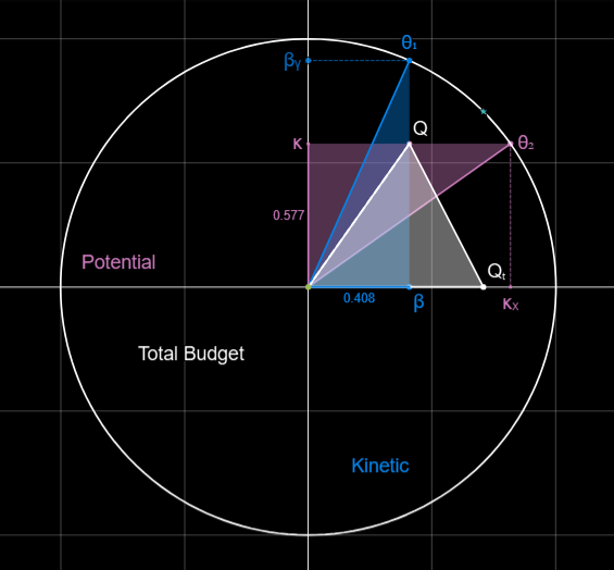
The Combined Energy Parameter \(Q\)
The total energy projection parameter unifies both aspects, describing the combined effects of relativity and gravity.
\(Q = \sqrt{\kappa^2 + \beta^2}\)
\(Q^{2} = 3\beta^2 = \frac{3}{2}\kappa^2 = \frac{3R_s}{2r}\)
\(Q_t = \sqrt{1-Q^2} = \sqrt{1-3\beta^2} = \sqrt{1-\frac{3}{2}\kappa^2}\)
\(Q_r = \frac{1}{Q_t}\)
Relativistic (\(\beta\)) and gravitational (\(\kappa\)) modes are dual aspects of one energy-transformation constraint.
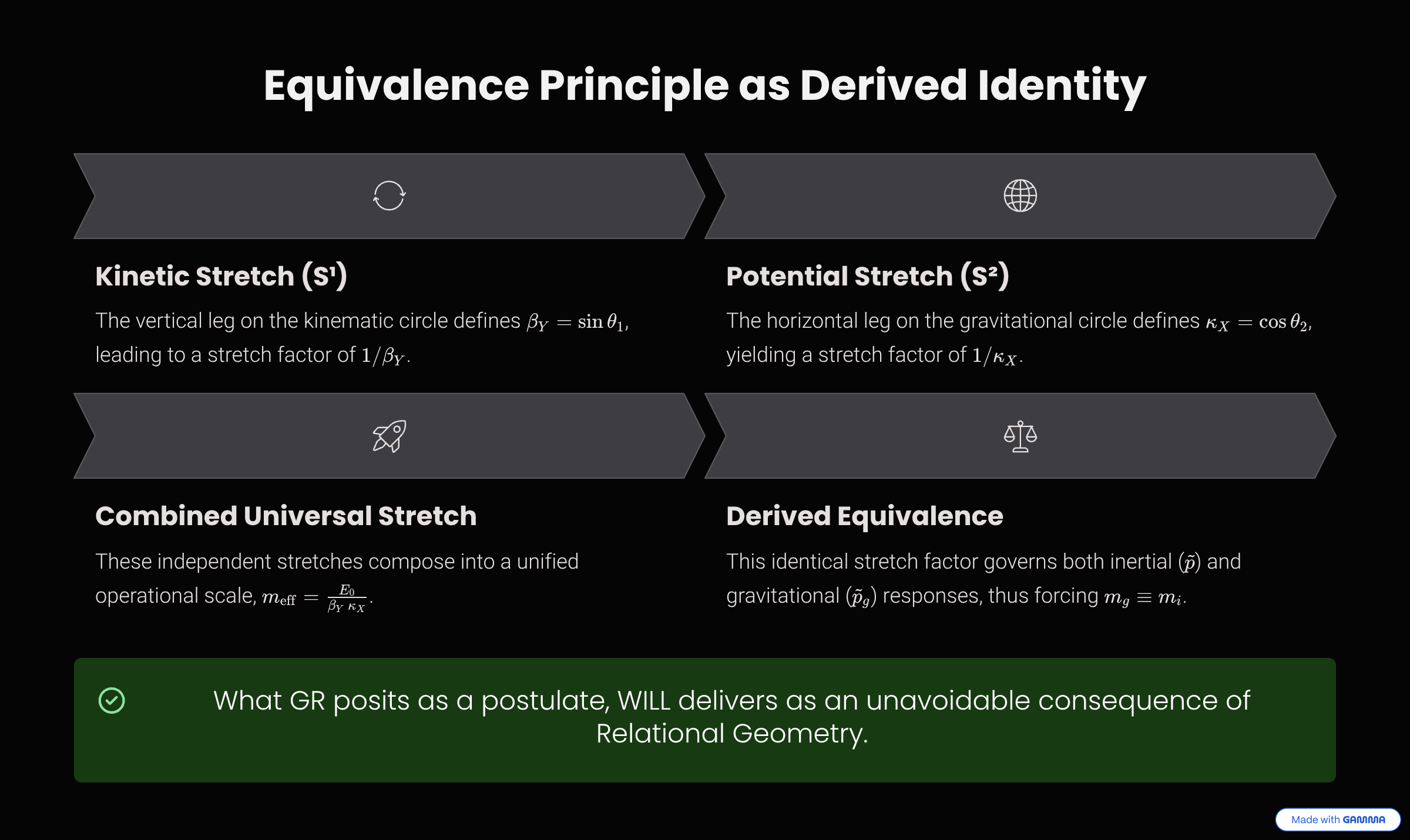
Equivalence Principle as a Derived Identity
In General Relativity, the Einstein Equivalence Principle is introduced as an independent postulate: \(m_g \equiv m_i\). Within WILL Geometry, no such axiom is required.
Composing the independent stretches from the kinematic (\(1/\beta_Y\)) and gravitational (\(1/\kappa_X\)) projections gives the total local energy:
\(E_{\text{loc}} = \frac{E_0}{\beta_Y \cdot \kappa_X} = \frac{E_0}{\sqrt{(1-\beta^2)(1-\kappa^2)}}\)
The inertial (\(\tilde p\)) and gravitational (\(\tilde p_g\)) projections share the same operational scale, governed by an identical effective mass factor, \(m_{\text{eff}}\). Hence, the equality is not assumed but is forced by the structure:
\(m_g \equiv m_i = m_{\text{eff}}\)
Remark on Eötvös-type precision
In WILL, the only invariant is \(E_0\), and the effective response is the universal stretch factor \(1/(\beta_Y\kappa_X)\). Since this factor depends solely on geometry and not on the composition of the test body, the universality of free fall follows by construction. What GR postulates, WILL reproduces as structural necessity.
What GR posits as a postulate, WILL delivers as an unavoidable consequence.
This derived equivalence is a profound consequence of composing the two projections. The framework's consistency, however, demands an even deeper connection: a precise 'exchange rate' that must exist between the kinetic and potential modes themselves.
Unification of Projections: The Geometric Exchange Rate
The Principle of a unified relational resource (Energy) requires a self-consistent "exchange rate" between its kinetic and potential modes. This rate is not an arbitrary parameter but is dictated by the intrinsic geometry of the relations themselves.
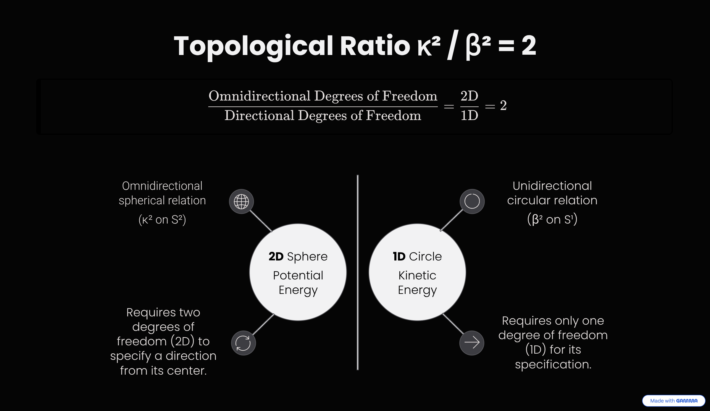
1. The Ratio of Relational Degrees of Freedom
An omnidirectional spherical relation (\(\kappa^2\) on \(S^2\)) requires two degrees of freedom (2D), while a directional circular relation (\(\beta^2\) on \(S^1\)) requires only one (1D). The intrinsic ratio is therefore 2. This is formally expressed as the ratio of their total solid angles:
\(\frac{\text{Total Closure of } S^2}{\text{Total Closure of } S^1} = \frac{4\pi}{2\pi} = 2\)
2. The Quadratic Nature of Energetic Realization
Energy is fundamentally quadratic in nature. The energetic significance of a state is proportional not to the amplitude of a projection (\(\beta\), \(\kappa\)), but to its square (\(\beta^2\), \(\kappa^2\)).
Proposition: Energetic Closure Criterion
In closed regimes, the unique quadratic balance compatible with directional (\(S^1\)) vs omnidirectional (\(S^2\)) resource splitting is:
\(\kappa^2=2\beta^2\)
The Principle as a Diagnostic Invariant
The relation \(\kappa^2 = 2\beta^2\) holds if the system is energetically closed (e.g., circular orbits). In open systems, its violation can be used to determine the magnitude of energy flow through unaccounted-for channels. When all channels are included, the equality is restored.
▶ Show Illustrative Examples
- Circular Orbit (Closed Subsystem): For a test body in a perfectly circular orbit, the condition \(\kappa^2 = 2\beta^2\) is exactly fulfilled. The system is energetically closed, and the equality signals full closure.
- Radiating Binary (Open Subsystem): For a binary system emitting gravitational waves, considering only orbital mechanics will show a violation of \(\kappa^2 = 2\beta^2\). This reveals the magnitude of energy flow through the unaccounted-for gravitational wave channel. When this channel is included in the balance, the equality holds again.
Geometric Distribution (\(\kappa^2\)) ≡ Kinetic Distribution (\(\beta^2\)) × 2
This topological ratio is the fundamental 'exchange rate' for energy within any closed system. It allows us to unify both kinetic and potential projections into a single, combined vector that describes the total energetic state of an object.
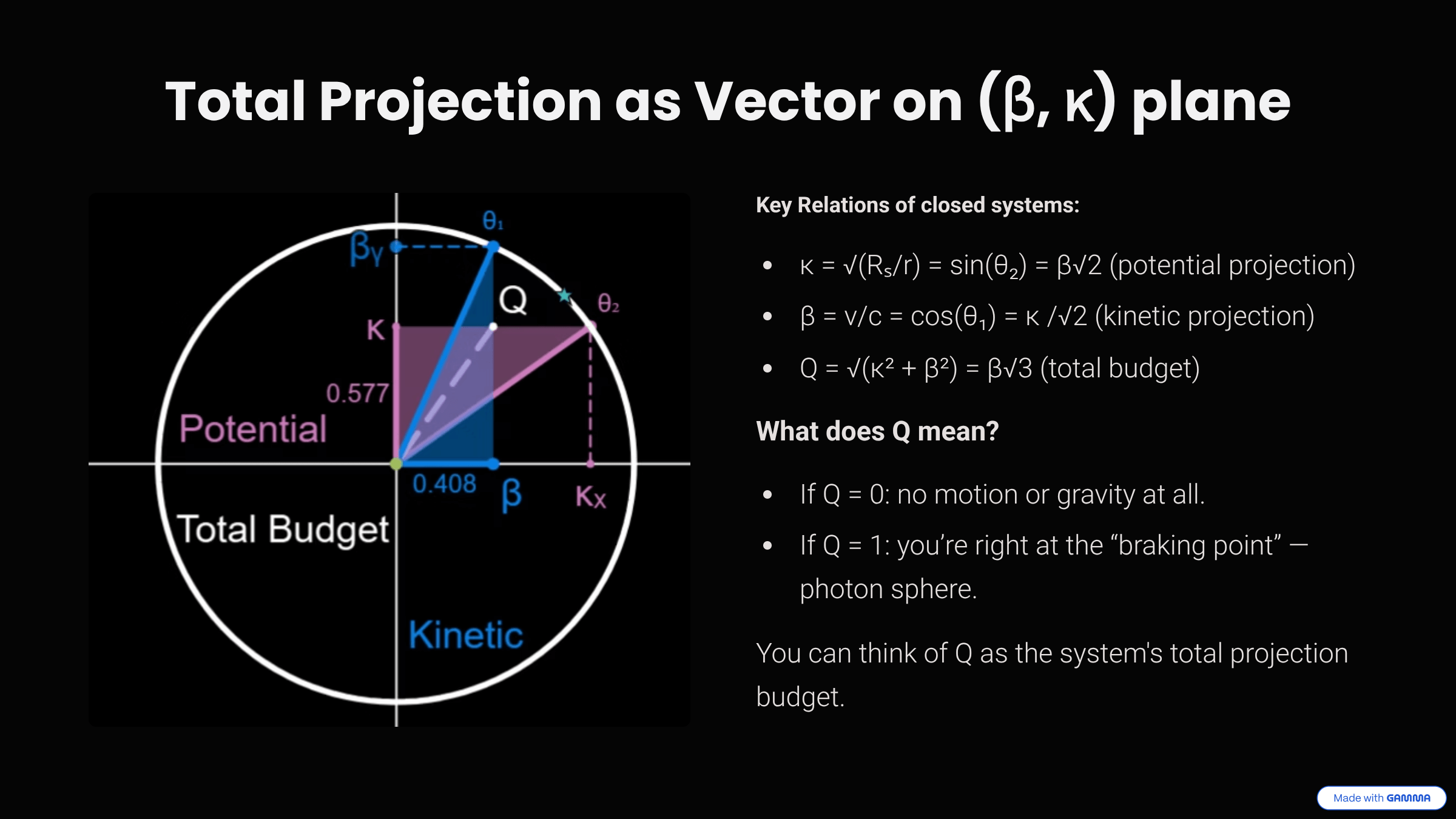
The Total Projection Parameter Q
▶ Show Interactive Graph: Q Circle (Desmos)
The combined effects of the kinetic (\(\beta\)) and potential (\(\kappa\)) projections are unified into a single vector, \(Q\), representing the system's total projection budget.
\(Q = \sqrt{\kappa^2 + \beta^2}\)
\(Q^{2} = 3\beta^2 = \frac{3}{2}\kappa^2\)
\(Q_t = \sqrt{1-Q^2}\)
This parameter describes the total energetic state of a closed system. Its boundary condition, \(Q=1\), corresponds to a critical state of the system—the photon sphere, where the geometry reaches its null-circumnavigation limit.
While the \(Q\) parameter describes the static geometric state of a system, transformations between states are governed by the framework's core dynamical rule: the Energy-Symmetry Law.
Energy as a Relation — What κ and β Actually Mean
Key Principle:
Energy isn’t something objects “have” — it’s a measure of differences between states.
When we drop anthropocentric distortions, a clear and intuitive picture emerges:
- Physical parameters like energy, speed, and gravitational potential don’t belong to objects.
- Instead, they represent how we, as observers, measure differences from our own point of view.
In this relational view, your perspective is always the reference frame. You are always at zero. Everything else is described by how it differs from your state:
- β (Beta) is not an intrinsic property of a moving object. It is a measure of how much of the universal “speed of change” you see as motion through space, relative to yourself.
- κ (Kappa) doesn’t describe an object’s “stored” gravitational energy. It measures how deeply an object sits in a gravitational field, as seen from your position. It’s your personal “ruler” for gravitational depth.
Think of κ and β as your own relational measuring tools:
- β is how far along your “motion ruler” you project another object’s state.
- κ is how deep into your “gravity well” you see another object’s state.
Energy thus emerges naturally:
- Energy is simply the capacity to move between states — it’s not possessed, but relationally defined.
- Saying “the object’s energy” always implicitly means “the object’s energy as measured from your perspective.”
Here’s a simple analogy:
Imagine standing on a train platform. A train passes by rapidly: to you, it has significant kinetic energy. But if you jump onto the train, it instantly becomes stationary relative to you. Its kinetic energy is now zero — because your frame of reference shifted. The energy didn’t vanish; your perspective changed.
Bottom line:
-
Energy, κ, and β aren’t hidden intrinsic qualities; they’re your personal, relational measurements.
-
All physics boils down to describing how things differ from your chosen point of view. No more, no less.
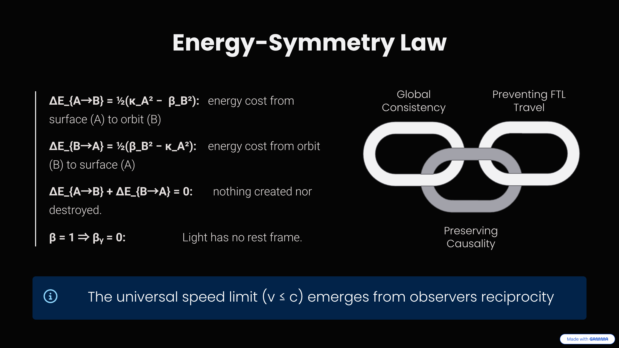
The Energy-Symmetry Law
Theorem: Energy Symmetry
The specific energy differences (per unit of rest energy) perceived by two observers for a transition between their states balance according to the Energy-Symmetry Law:
\(\Delta E_{A \to B} + \Delta E_{B \to A} = 0\)
Proof
Consider observer A at rest (\(\beta_A=0\)) on a surface with potential \(\kappa_A\), and observer B in an orbit with potential \(\kappa_B\) and velocity \(\beta_B\). The total specific energy for the transition \(A \to B\) is the sum of the change in potential and kinetic energy budgets:
\(\Delta E_{A \to B} = \frac{1}{2}\left((\kappa_A^2 - \kappa_B^2) + \beta_B^2\right)\)
From B's perspective, the transition \(B \to A\) yields:
\(\Delta E_{B \to A} = \frac{1}{2}\left((\kappa_B^2 - \kappa_A^2) - \beta_B^2\right)\)
Summing these transfers gives \(\Delta E_{A \to B} + \Delta E_{B \to A} = 0\). No net energy is created or destroyed in a closed cycle of transitions.
Universal Speed Limit as a Consequence
Theorem: Universal Speed Limit
The universal speed limit (\(v \leq c\)) emerges from the requirement of energetic symmetry.
Proof
Assume an object could exceed the speed of light, implying \(\beta > 1\). The energy transfer required, \(\Delta E_{A \to B}\), would become arbitrarily large. Consequently, no finite physical process could provide a balancing reverse transfer, \(\Delta E_{B \to A}\), that would sum to zero. The fundamental symmetry would be broken. Therefore, the condition \(\beta \leq 1\) is an intrinsic requirement for maintaining the causal and energetic consistency of the relational universe.
Single-Axis Energy Transfer and the Nature of Light
Theorem: Single-Axis Transformation Principle
For light, the kinematic projection reaches its full extent: \(\beta = 1 \Rightarrow \beta_Y = 0\). All transformation of the relational energy occurs along a single orthogonal axis.
Proof
For massive systems, the energy exchange is distributed between two orthogonal projections. For light, \(\beta_Y = 0\), so the complementary projection disappears. The full relational resource is realized on a single projection. Therefore, the specific energy potential for light is not halved but complete, \(\Phi_\gamma = \kappa^2 c^2\), while for a massive body it remains partitioned, \(\Phi_{\text{mass}} = \frac{1}{2}\kappa^2 c^2\). This explains why light experiences a geometric effect exactly twice that of a massive particle in the same field.
▶ Show Simplification for Closed Orbits
When the closure condition for stable orbits (\(\kappa^2 = 2\beta^2\)) is applied, the general law simplifies.
-
Surface-to-Orbit Transfer: The specific energy balance is given by:
\(\frac{E_{A \to B}}{E_{0B}} = \frac{1}{2}(\kappa_A^2 - \beta_B^2)\) -
Orbit-to-Orbit Transfer: The balance reduces further, with the potential terms cancelling out completely:
\(\frac{E_{A \to B}}{E_{0B}} = \frac{1}{2}(\beta_A^2 - \beta_B^2)\)
Causality is a built-in feature of Relational Geometry.
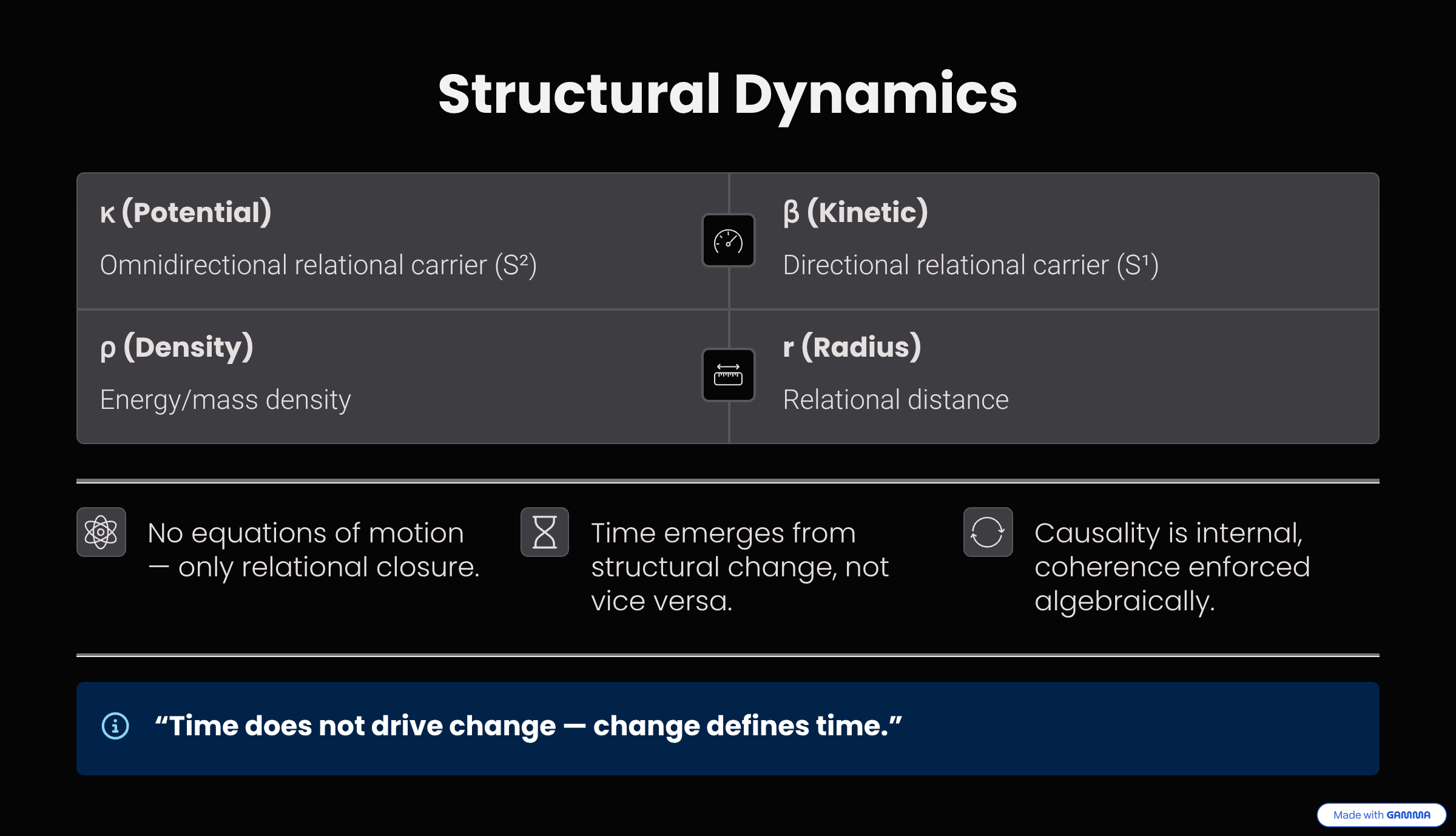
Beyond Differential Formalism: Structural Dynamics
The system is not described by differential equations of motion evolving in time. Instead, its transformation is dictated by a closed network of algebraic relations that enforce a perpetually balanced configuration. What we perceive as "dynamics" is this ordered succession of balanced states.
Time does not drive change — change defines time.
Time as an Emergent Property
In this framework, time is not a fundamental entity but a derived concept tied to changes in the system's geometry. Similar to time dilation, time intervals here are defined by the transformations of geometric parameters like \(r\) and \(\kappa\). A natural time scale arises from the geometry as \(t_{d} = r/c\). This intrinsic time scale encapsulates the system's dynamics without invoking an independent time variable.
Algebraic Closure and Structural Causality
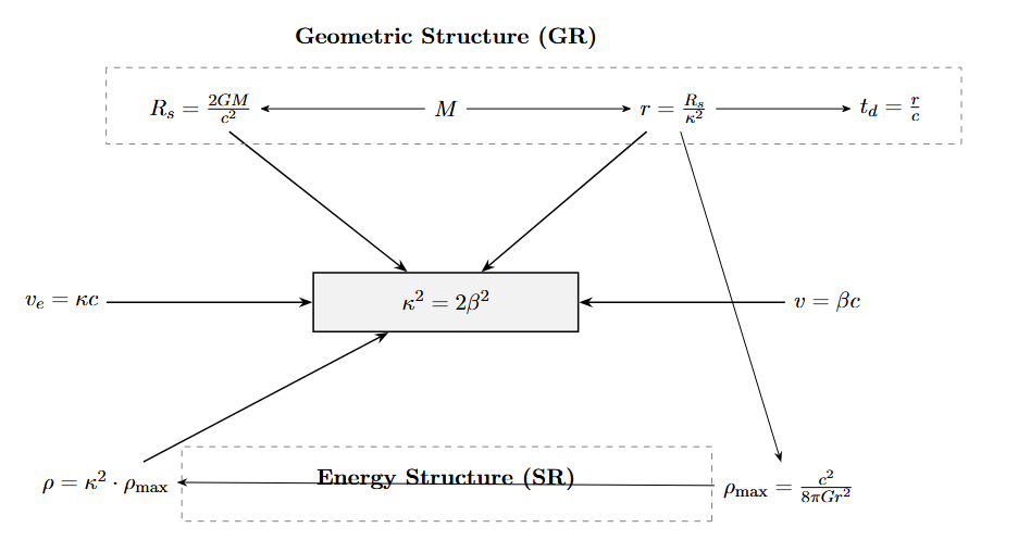
Physical dynamics emerges from a set of algebraically closed invariants. Each parameter participates in a self-consistent configuration of relational constraints. Changing any one parameter necessitates a coordinated shift in all others to maintain validity. The following set of relations expresses this minimal algebraic closure:
\(\kappa^2 = 2 \beta^2\)
\(r \cdot \kappa^2 = R_s \quad \text{where} \quad R_s = \frac{2G m_0}{c^2}\)
\(\rho = \frac{\kappa^2 c^2}{8\pi Gr^2}\)
\(m_0 = 4\pi r^3 \cdot \rho\)
▶ Show Comparison with Classical Dynamics
Why There Are No Equations of Motion
Classical physics formulates dynamics through differential equations (Lagrangians, variational principles), assuming a continuum of paths where nature selects one by minimizing action. WILL Geometry begins from a different premise: there is no "space" of possible paths and no "freedom to vary." The system does not evolve through time; it defines time through its structure. There is only one valid configuration at any moment: the one where all projectional constraints are satisfied.
▶ Show a Numerical Example
Accretion onto a Black Hole
Consider a black hole of \(10 M_\odot\) accreting mass. Let \(\kappa = 0.1\). The initial radius is \(r = R_s/\kappa^2 = 2.95 \times 10^6\) m, and the time scale is \(t_d = r/c \approx 9.83\) ms. As it accretes mass to \(10.1 M_\odot\), its \(R_s\) increases. Assuming \(\kappa\) remains constant, the radius \(r\) and the time scale \(t_d\) adjust accordingly to \(2.98 \times 10^6\) m and \(9.93\) ms. This increase in \(t_d\) reflects the system's evolution, driven solely by the changing geometry without differential equations.
Dynamics is the ordered succession of balanced configurations.
This principle of structural dynamics culminates in the framework's central equation, which unifies geometry and energy density into a single, profound statement.
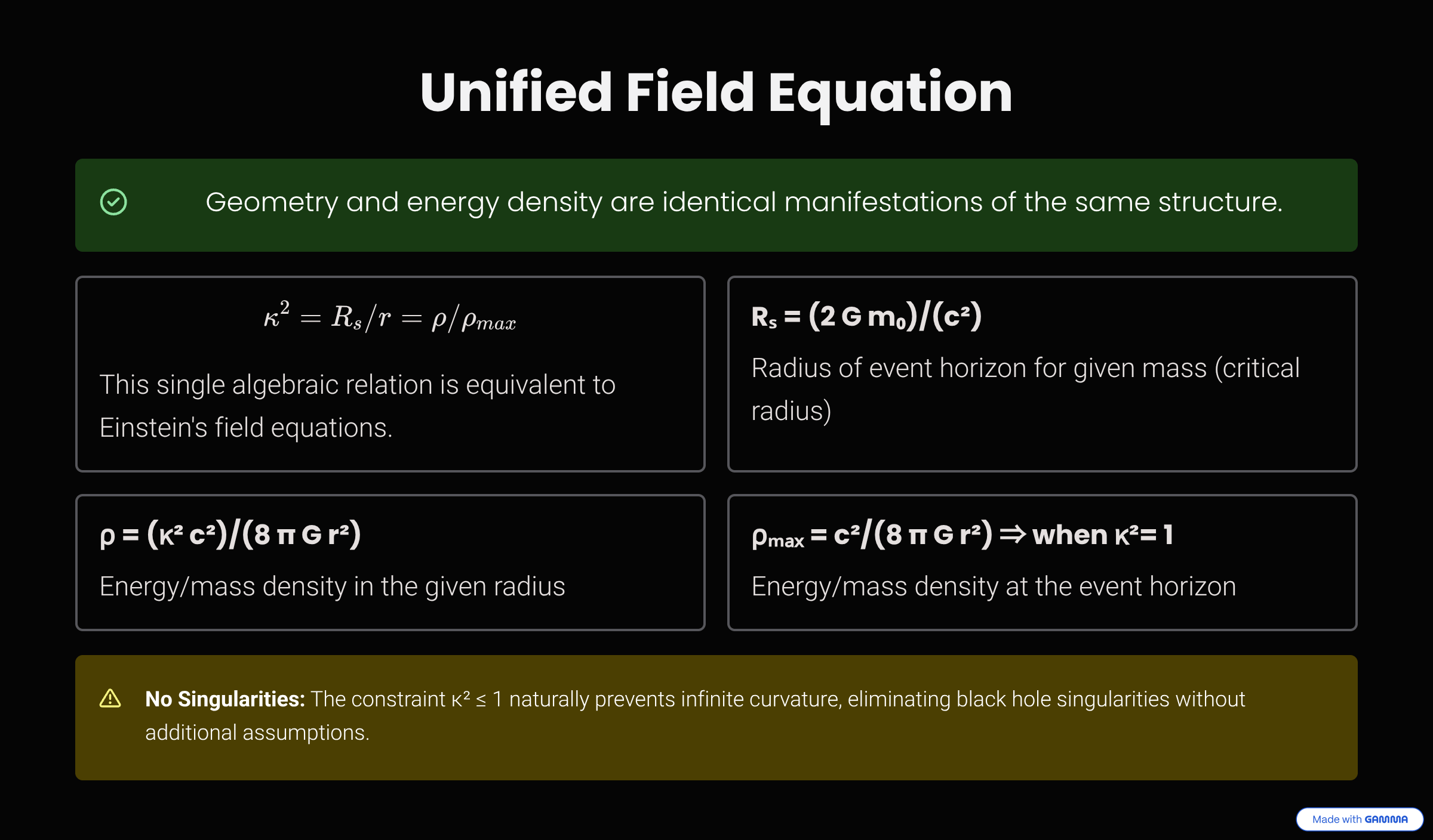
The Unified Field Equation
From the energy-geometry equivalence, the complete description of gravitational phenomena reduces to a single algebraic relation. This equation expresses the core identity: the ratio of geometric scales equals the ratio of energy densities.
\(\kappa^2 = \frac{R_s}{r} = \frac{\rho}{\rho_{\text{max}}}\)
This single algebraic relation is the unified field equation of WILL Geometry. It ensures that curvature and energy density evolve smoothly and remain bounded, resolving the singularity problem by geometrically constraining the domain of valid projections.
▶ Show Formal Derivation of Energy Density
Geometric Foundation
From the projective analysis, the fundamental invariant is \(\kappa^2 = R_s/r\), where \(R_s = 2Gm_0/c^2\).
Derivation of Energy Density (\(\rho\))
Starting from the geometric relation \(m_0 = \frac{\kappa^2 c^2 r}{2G}\), we associate \(m_0\) with a volumetric proxy \(r^3\). Because the potential projection \(\kappa\) is distributed over a 2D spherical manifold (\(S^2\)), the expression must be normalized over the unit-sphere area \(4\pi\). This yields the physical energy density:
\(\rho = \frac{1}{4\pi}\left(\frac{\kappa^2 c^2}{2G r^2}\right) = \frac{\kappa^2c^2}{8\pi G r^2}\)
Maximal Density (\(\rho_{\text{max}}\))
At the horizon condition, \(\kappa^2 = 1\), the maximal observable energy density at radius \(r\) is reached:
\(\rho_{\text{max}} = \frac{c^2}{8\pi G r^2}\)
Thus, the fundamental identification is \(\kappa^2 = \rho/\rho_{\text{max}}\).
No Singularities: The constraint \(\kappa^2 \le 1\) naturally prevents infinite curvature.
This equation closes the theoretical loop, demonstrating that the framework's foundational principle is proven as the inevitable consequence of its own geometric consistency—a concept best visualized as the Theoretical Ouroboros.
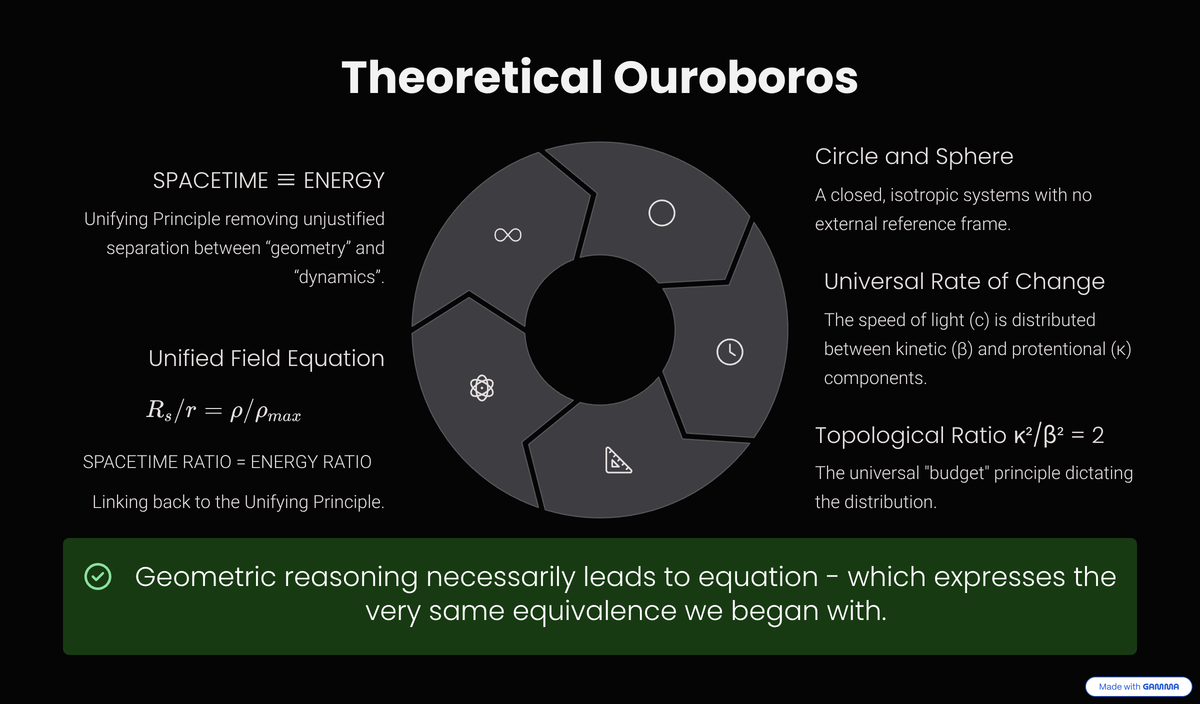
The Theoretical Ouroboros
The Unified Field Equation closes the theoretical loop. The single foundational principle, through pure geometric reasoning, necessarily leads to an equation which mathematically expresses the very same equivalence we began with.
The initial principle \(\text{SPACETIME} \equiv \text{ENERGY}\) logically derives the geometry and physical laws, and these derived laws then loop back to intrinsically define and prove the self-consistency of the initial idea.
The WILL framework exhibits perfect logical closure: the fundamental principle is proven as the inevitable consequence of geometric consistency.
This logical closure is elegant, but a physical theory is only as strong as its empirical predictions. The final step is to ground this abstract framework in real-world, measurable phenomena.
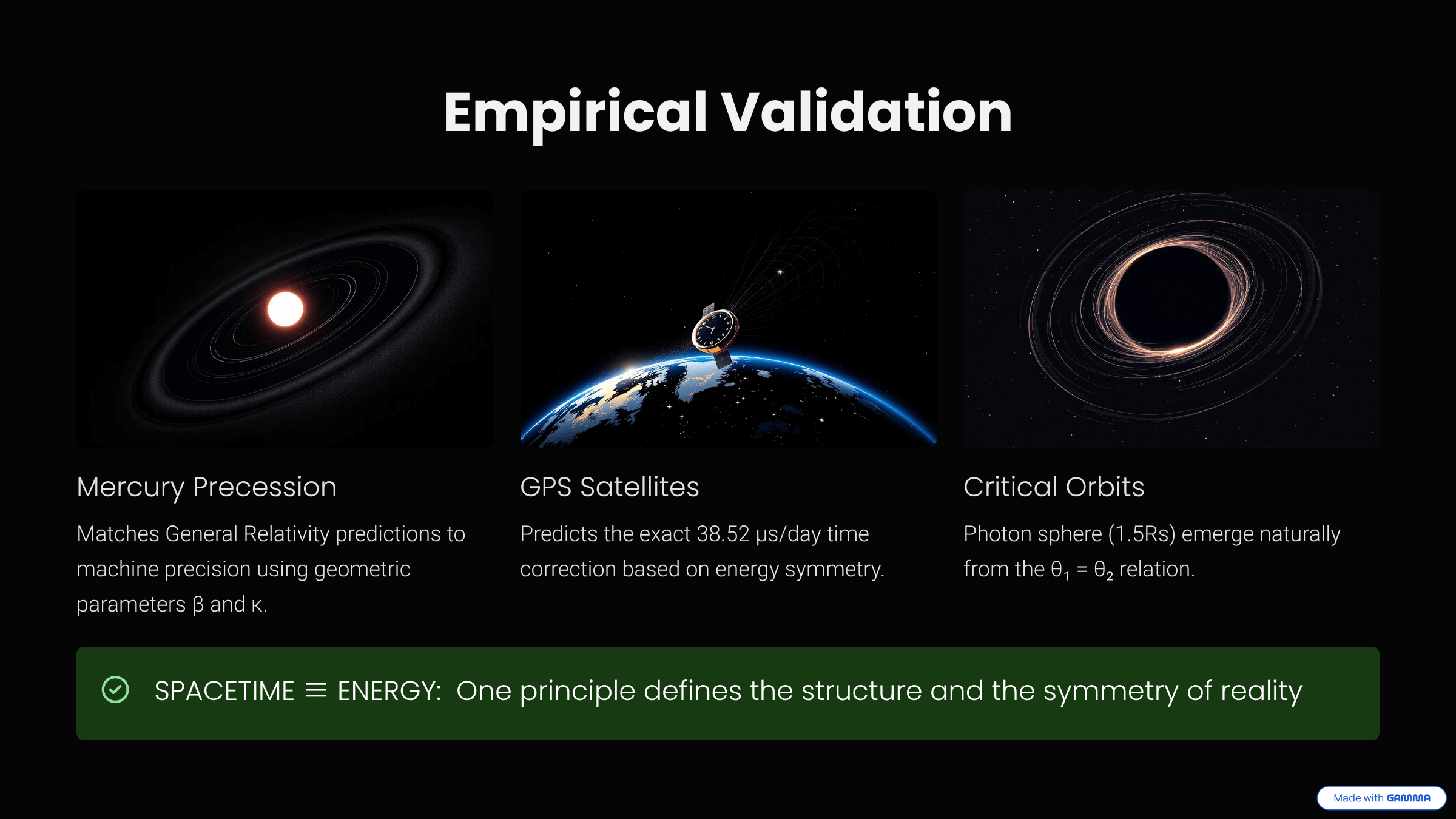
Grounding the Vision in Reality
A theory born of pure logic must find its reflection in the workings of the real world. WILL Relational Geometry passes rigorous experimental and observational tests, reproducing the successes of standard physics from deeper, more unified first principles.
Critical Orbits (ISCO & Photon Sphere)
All known GR critical surfaces emerge naturally from the geometric equilibrium of the \(\beta\) and \(\kappa\) projections, without solving geodesic equations.
▶ Show Derivation of Critical Orbits
Geometric Prediction of Photon Sphere and ISCO
Critical orbital radii emerge not from solving complex geodesic equations, but as direct consequences of fundamental symmetries within the projection budget \(Q\).
1. Photon Sphere from the Principle of Maximum Projection (\(Q=1\))
The Photon Sphere represents a state of maximum geometric saturation, where the entire projection budget is exhausted. This is expressed by the symmetry condition:
\(Q = 1 \implies Q^2 = 1\)
Using the system's definitions (\(Q^2 = \kappa^2 + \beta^2\)) and the universal law for closed systems (\(\kappa^2 = 2\beta^2\)), we solve:
\(2\beta^2 + \beta^2 = 1 \implies 3\beta^2 = 1 \implies \beta^2 = \frac{1}{3}\)
\(\kappa^2 = 2\beta^2 = \frac{2}{3}\)
From the definition \(r = R_s / \kappa^2\), we derive the physical radius:
\(r_{ps} = \frac{R_s}{2/3} = 1.5 R_s\)
2. ISCO from the Principle of Equilibrium (\(Q=Q_t\))
The Innermost Stable Circular Orbit (ISCO) represents a state of perfect equilibrium, where the "used" projection budget (\(Q\)) equals the "complementary" budget (\(Q_t=\sqrt{1-Q^{2}}\)). This symmetry of marginal stability is expressed as:
\(Q = Q_t \implies Q^2 = Q_t^2\)
Using the definition \(Q_t^2 = 1 - Q^2\), we solve for \(Q^2\):
\(Q^2 = 1 - Q^2 \implies 2Q^2 = 1 \implies Q^2 = \frac{1}{2}\)
Again, using the system's law (\(\kappa^2 = 2\beta^2\)) and definitions (\(Q^2 = \kappa^2 + \beta^2\)), we solve:
\(2\beta^2 + \beta^2 = \frac{1}{2} \implies 3\beta^2 = \frac{1}{2} \implies \beta^2 = \frac{1}{6}\)
\(\kappa^2 = 2\beta^2 = \frac{1}{3}\)
From \(r = R_s / \kappa^2\), we derive the physical radius:
\(r_{isco} = \frac{R_s}{1/3} = 3 R_s\)
While the radii are known from GR, their emergence from two distinct, symmetries (\(Q=1\) and \(Q=Q_t\)) reinforces the explanatory power of Relational Geometry.
GPS Satellites
The model correctly predicts the empirically measured time correction by unifying kinetic (SR) and gravitational (GR) effects into a single calculation.
▶ Show Interactive Graph: Earth GPS (Desmos)
▶ Show Full Calculation for GPS Time Shift
Using the combined time factor \(\tau = \beta_Y \cdot \kappa_X\), we calculate the daily relativistic offset between GPS satellite clocks and Earth-based clocks.
\(\beta_{GPS} = 0.0000129... \Rightarrow \beta_{YGPS} = 0.999999999917\)
\(\kappa_{GPS} = 0.0000182... \Rightarrow \kappa_{XGPS} = 0.999999999833\)
\(\tau_{GPS} = \kappa_{XGPS} \cdot \beta_{YGPS} = 0.99999999975\)
\(\kappa_{Earth} = 0.0000373... \Rightarrow \kappa_{XEarth} = 0.999999999304\)
\(\tau_{Earth} = \kappa_{XEarth} \cdot 1 = 0.999999999304\)
\(\Delta \tau = (1-\frac{\tau_{Earth}}{\tau_{GPS}}) \cdot 86400 \cdot 10^6\)
\(\Delta \tau \approx 38.52 \text{ µs/day}\)
This result exactly matches the empirical time correction required for GPS synchronization and confirms the Energy-Symmetry Law using real-world data.
Mercury Precession
The theory computes the anomalous precession of Mercury’s orbit, matching the observed data with machine-level precision.
▶ Show Full Calculation for Mercury's Precession
▶ Show Interactive Graph: Sun–Mercury (Desmos)
The precession is calculated from the combined energy parameter \(Q^2\) and orbital eccentricity \(e\).
\(\kappa_{Merc} = 0.000225...\)
\(\beta_{Merc} = 0.000159...\)
\(Q_{Merc}^2 = 3 \beta_{Merc}^2 = 7.653... \times 10^{-8}\)
\(\Delta\phi_{WILL} = \frac{2\pi Q_{Merc}^{2}}{(1-e_{Merc}^{2})} = 5.02087... \times 10^{-7}\) radians
\(\Delta\phi_{GR} = \frac{3\pi R_{Ssun}}{a_{Merc} (1 - e_{Merc}^{2})} = 5.02087... \times 10^{-7}\) radians
Relative Difference: \(< 10^{-9}\) %
The negligible difference confirms that WILL Geometry reproduces the observed relativistic precession of Mercury to within machine accuracy.
SPACETIME ≡ ENERGY: One principle defines the structure and the symmetry of reality.
The Name "WILL"
The name Will reflects both the harmonious unity between structure and dynamics and a subtle irony towards the anthropic principle, which often intertwines human existence with the causality of the universe. This model stands as a testament to the universal laws of physics, transcending any anthropocentric framework.
The World as a Projection
This exploration is only the beginning. The model has been extended to cover cosmology and quantum mechanics, with further results and detailed applications available below. The core idea remains: energy does not exist in spacetime—it creates spacetime by its projection.